Hallo

Figure 1 illustrates different things. Figure 1 (a) illustrates this, Figure 1 (b) illustrates that and so on

library(ggplot2)
ggplot(mtcars,
       aes(mpg, hp, size = gear)) +
  geom_point()

ggplot(mtcars,
       aes(mpg, hp, size = gear)) +
  geom_point() + 
  geom_smooth()

ggplot(mtcars,
       aes(mpg, hp, size = gear)) +
  geom_point() + 
  geom_smooth(method = "lm")
ggplot(mtcars,
       aes(mpg, hp, size = gear)) +
  geom_point() + 
  geom_smooth(method = "glm", method.args = list(family = "poisson"))

(a) The data

(b) Polynomial

(c) Linear Model

(d) GLM with Poisson

Figure 1: One dataset, different models

ggplot(mtcars, 
       aes(hp, mpg, color = factor(am))) +
  geom_point() +
  geom_smooth(formula = y ~ x, method = "loess") +
  theme(legend.position = 'bottom')
datatable(mtcars,
  options = list(pageLength = 5))

library(kableExtra)
kable(head(cars))
kable(head(pressure))

Table 1: Datasets

(a) Cars

speed	dist
4	2
4	10
7	4
7	22
8	16
9	10

(b) Pressure

temperature	pressure
0	0.0002
20	0.0012
40	0.0060
60	0.0300
80	0.0900
100	0.2700

data =read.csv('data/dataset.csv')

head = data

class(data)

[1] "data.frame"

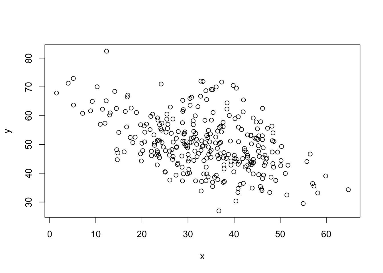
x = data$anxiety
y= data$flexibility
plot(x, y)

summary(data)

    anxiety        flexibility    mindfulness          activity        
 Min.   : 1.483   Min.   :26.91   Length:300         Length:300        
 1st Qu.:25.977   1st Qu.:44.24   Class :character   Class :character  
 Median :33.922   Median :49.56   Mode  :character   Mode  :character  
 Mean   :33.418   Mean   :50.34                                        
 3rd Qu.:41.974   3rd Qu.:56.32                                        
 Max.   :64.775   Max.   :82.41                                        

sum(is.na(data))

[1] 0

Figure 2 illustrates a plot

knitr::include_graphics("images/table.png")

Figure 2: Fig. motor transfer between expert and nonathlets

Table 2 illustrates a table

```{r}
#| label: tbl-motor 
#| tbl-cap: "Iris Data"
library(kableExtra)
kable(mtcars) %>%
  scroll_box(height = "450px", width = "100%")
```

Table 2: Iris Data

	mpg	cyl	disp	hp	drat	wt	qsec	vs	am	gear	carb
Mazda RX4	21.0	6	160.0	110	3.90	2.620	16.46	0	1	4	4
Mazda RX4 Wag	21.0	6	160.0	110	3.90	2.875	17.02	0	1	4	4
Datsun 710	22.8	4	108.0	93	3.85	2.320	18.61	1	1	4	1
Hornet 4 Drive	21.4	6	258.0	110	3.08	3.215	19.44	1	0	3	1
Hornet Sportabout	18.7	8	360.0	175	3.15	3.440	17.02	0	0	3	2
Valiant	18.1	6	225.0	105	2.76	3.460	20.22	1	0	3	1
Duster 360	14.3	8	360.0	245	3.21	3.570	15.84	0	0	3	4
Merc 240D	24.4	4	146.7	62	3.69	3.190	20.00	1	0	4	2
Merc 230	22.8	4	140.8	95	3.92	3.150	22.90	1	0	4	2
Merc 280	19.2	6	167.6	123	3.92	3.440	18.30	1	0	4	4
Merc 280C	17.8	6	167.6	123	3.92	3.440	18.90	1	0	4	4
Merc 450SE	16.4	8	275.8	180	3.07	4.070	17.40	0	0	3	3
Merc 450SL	17.3	8	275.8	180	3.07	3.730	17.60	0	0	3	3
Merc 450SLC	15.2	8	275.8	180	3.07	3.780	18.00	0	0	3	3
Cadillac Fleetwood	10.4	8	472.0	205	2.93	5.250	17.98	0	0	3	4
Lincoln Continental	10.4	8	460.0	215	3.00	5.424	17.82	0	0	3	4
Chrysler Imperial	14.7	8	440.0	230	3.23	5.345	17.42	0	0	3	4
Fiat 128	32.4	4	78.7	66	4.08	2.200	19.47	1	1	4	1
Honda Civic	30.4	4	75.7	52	4.93	1.615	18.52	1	1	4	2
Toyota Corolla	33.9	4	71.1	65	4.22	1.835	19.90	1	1	4	1
Toyota Corona	21.5	4	120.1	97	3.70	2.465	20.01	1	0	3	1
Dodge Challenger	15.5	8	318.0	150	2.76	3.520	16.87	0	0	3	2
AMC Javelin	15.2	8	304.0	150	3.15	3.435	17.30	0	0	3	2
Camaro Z28	13.3	8	350.0	245	3.73	3.840	15.41	0	0	3	4
Pontiac Firebird	19.2	8	400.0	175	3.08	3.845	17.05	0	0	3	2
Fiat X1-9	27.3	4	79.0	66	4.08	1.935	18.90	1	1	4	1
Porsche 914-2	26.0	4	120.3	91	4.43	2.140	16.70	0	1	5	2
Lotus Europa	30.4	4	95.1	113	3.77	1.513	16.90	1	1	5	2
Ford Pantera L	15.8	8	351.0	264	4.22	3.170	14.50	0	1	5	4
Ferrari Dino	19.7	6	145.0	175	3.62	2.770	15.50	0	1	5	6
Maserati Bora	15.0	8	301.0	335	3.54	3.570	14.60	0	1	5	8
Volvo 142E	21.4	4	121.0	109	4.11	2.780	18.60	1	1	4	2

Listing 1: Basic use of the plot() function

plot(cars)

Listing 1 illustrates a basic use of the function plot()

Equation 1 illustrates how to standardize a value \[ z = \frac{x_i - \bar{x}}{s} \tag{1}\]

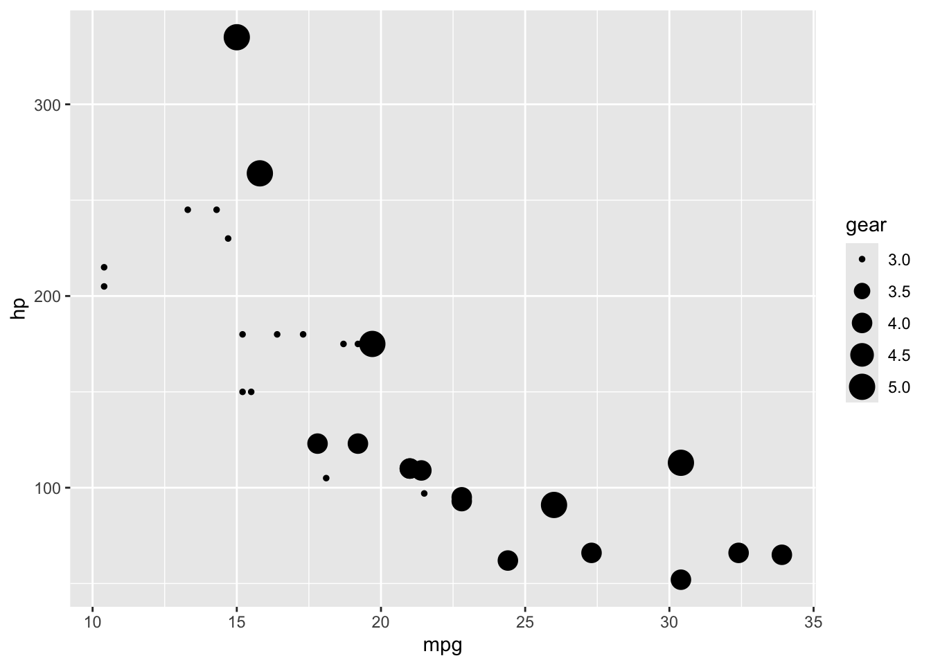
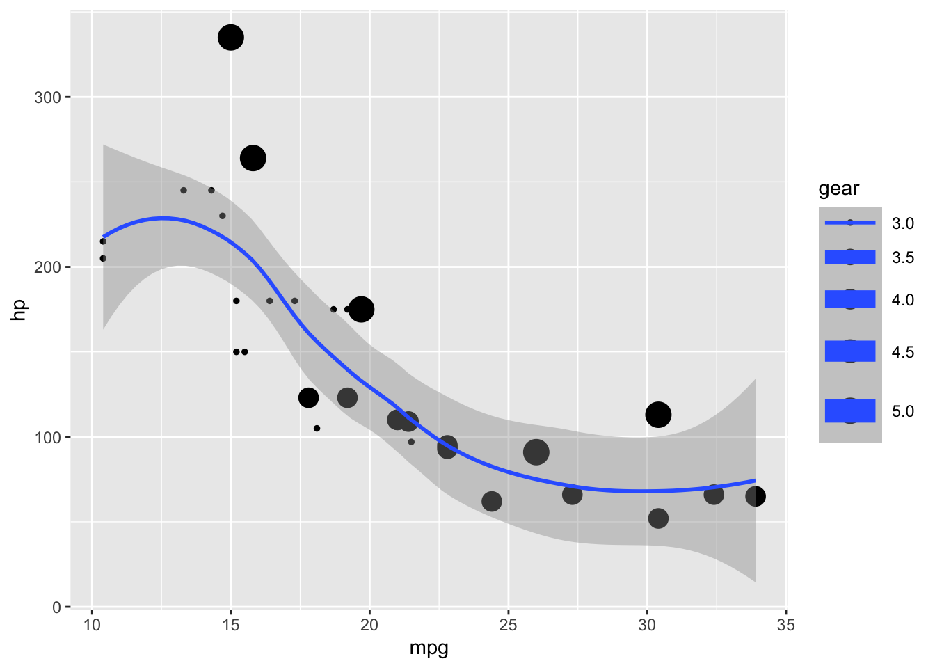
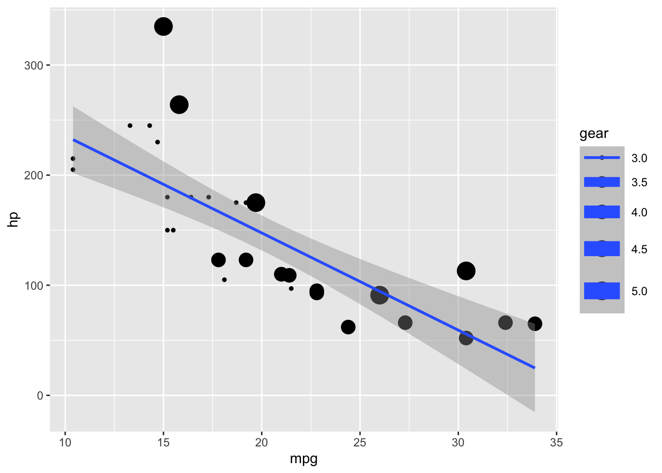
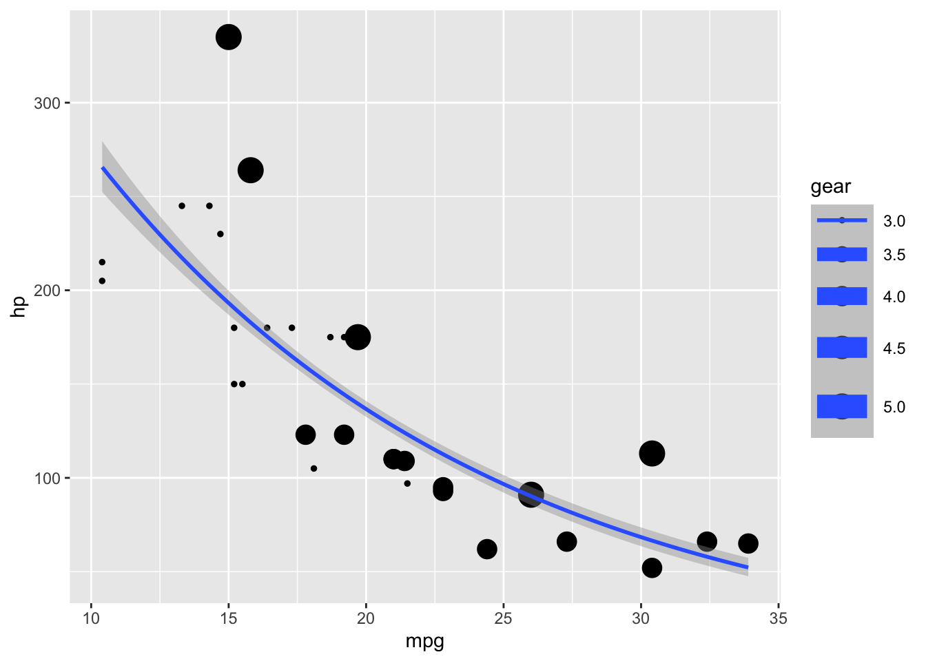
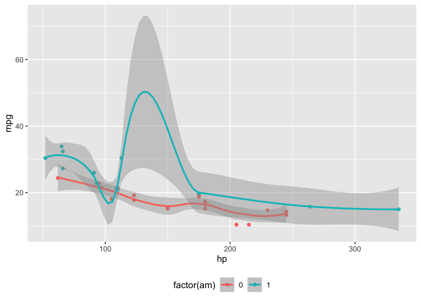
library(ggplot2)
#| out-width: 80%                                
#| fig-align: right                            
#| fig-cap: A graph from `mtcars`
#| fig-cap-location: bottom
#| label: fig-mtcars1
ggplot(mtcars, aes(hp, mpg, color = factor(am))) +
  geom_point() +
  geom_smooth(formula = y ~ x, method = "loess") +
  theme(legend.position = 'bottom')

ggplot2 is an R (R Core Team 2025) package developed by (Wickham 2016). Epifania, Anselmi, and Robusto (2024) published an interesting paper on Linear Mixed Effects Models.

R Core Team. 2025. R: A Language and Environment for Statistical Computing. Vienna, Austria: R Foundation for Statistical Computing. https://www.R-project.org/.

Wickham, Hadley. 2016. Ggplot2: Elegant Graphics for Data Analysis. Springer-Verlag New York. https://ggplot2.tidyverse.org.

Epifania, Ottavia M, Pasquale Anselmi, and Egidio Robusto. 2024. “A Guided Tutorial on Linear Mixed-Effects Models for the Analysis of Accuracies and Response Times in Experiments with Fully Crossed Design.” Psychological Methods. https://doi.org/https://doi.org/10.1037/met0000708.

I want this picture displayed in the margin

eeg!

fnirs!

Aim

the nature of neuroplacity in human

Methods

behavior, fnirs, eeg, tdcs

Results

the brain support the motor learning

First level

I miss you.

Second level

I miss you.

Third level

i DO MISS you

Fourth level

I do do do do miss you

Hahahahaha

Frankly² speaking, i do not miss you

My researchgate is here

welcome to the phd

This is science.

this is his image

Note

To say something general

I’m a title!

Maybe a tip :)

Pay attention!

Please pay attention to whatever it is written here

Warning

Just saying you should be careful

5*5

[1] 25

5^2

[1] 25

#|echo: true
1mtcars %>%
2  ggplot( aes(mpg, hp, size = gear)) +
3  geom_point() +
4  geom_smooth(method = "lm")

1

This does that

2

This other thing is this

3

And look at this!

4

Please have mercy